7  Procedimentos Gráficos

7.1 Introdução ao ggplot2

O ggplot2 é uma das bibliotecas mais populares para criação de gráficos em R. Ele foi desenvolvido por Hadley Wickham e é conhecido por sua abordagem de “gramática dos gráficos”, que permite criar visualizações complexas com facilidade. Uma das principais características do ggplot2 é o conceito de camadas, onde adicionamos componentes visuais ao gráfico de forma incremental, permitindo maior controle sobre a estética e os dados representados.

Para começar a trabalhar com o ggplot2, precisamos carregar a biblioteca, o ggplot2 faz parte do tidyverse.

Para a aula de hoje, vamos agrupar 16 bancos de dados sobre “Filmes”, disponíveis em Kaggle.

Primeira coisa que precisamos fazer é ler os 16 bancos de dados, criar uma variável com o tipo do filme e em seguida montar o nosso banco único para podermos explorar os dados.

• Lendo os dados

require(data.table)

Loading required package: data.table

require(tidyverse)

Loading required package: tidyverse

── Attaching core tidyverse packages ──────────────────────── tidyverse 2.0.0 ──
✔ dplyr     1.1.4     ✔ readr     2.1.5
✔ forcats   1.0.0     ✔ stringr   1.5.1
✔ ggplot2   3.5.1     ✔ tibble    3.2.1
✔ lubridate 1.9.3     ✔ tidyr     1.3.1
✔ purrr     1.0.2     
── Conflicts ────────────────────────────────────────── tidyverse_conflicts() ──
✖ dplyr::between()     masks data.table::between()
✖ dplyr::filter()      masks stats::filter()
✖ dplyr::first()       masks data.table::first()
✖ lubridate::hour()    masks data.table::hour()
✖ lubridate::isoweek() masks data.table::isoweek()
✖ dplyr::lag()         masks stats::lag()
✖ dplyr::last()        masks data.table::last()
✖ lubridate::mday()    masks data.table::mday()
✖ lubridate::minute()  masks data.table::minute()
✖ lubridate::month()   masks data.table::month()
✖ lubridate::quarter() masks data.table::quarter()
✖ lubridate::second()  masks data.table::second()
✖ purrr::transpose()   masks data.table::transpose()
✖ lubridate::wday()    masks data.table::wday()
✖ lubridate::week()    masks data.table::week()
✖ lubridate::yday()    masks data.table::yday()
✖ lubridate::year()    masks data.table::year()
ℹ Use the conflicted package (<http://conflicted.r-lib.org/>) to force all conflicts to become errors

require(magrittr)

Loading required package: magrittr

Attaching package: 'magrittr'

The following object is masked from 'package:purrr':

    set_names

The following object is masked from 'package:tidyr':

    extract

files = system("ls ../data/movies", intern = TRUE)

filmes = list()
for(i in 1:length(files)){
  nome = gsub(x = files[i], 
              pattern = ".csv", 
              replacement = "")
  
  filmes[[i]] <- fread(paste0("../data/movies/",  files[i])) %>% 
    mutate(tipo = nome)
  
  filmes[[i]]$year %<>% as.integer()
  filmes[[i]]$`gross(in $)` %<>% as.numeric()
  
}

Warning in filmes[[i]]$year %<>% as.integer(): NAs introduced by coercion
Warning in filmes[[i]]$year %<>% as.integer(): NAs introduced by coercion
Warning in filmes[[i]]$year %<>% as.integer(): NAs introduced by coercion
Warning in filmes[[i]]$year %<>% as.integer(): NAs introduced by coercion
Warning in filmes[[i]]$year %<>% as.integer(): NAs introduced by coercion
Warning in filmes[[i]]$year %<>% as.integer(): NAs introduced by coercion
Warning in filmes[[i]]$year %<>% as.integer(): NAs introduced by coercion
Warning in filmes[[i]]$year %<>% as.integer(): NAs introduced by coercion
Warning in filmes[[i]]$year %<>% as.integer(): NAs introduced by coercion
Warning in filmes[[i]]$year %<>% as.integer(): NAs introduced by coercion
Warning in filmes[[i]]$year %<>% as.integer(): NAs introduced by coercion
Warning in filmes[[i]]$year %<>% as.integer(): NAs introduced by coercion
Warning in filmes[[i]]$year %<>% as.integer(): NAs introduced by coercion
Warning in filmes[[i]]$year %<>% as.integer(): NAs introduced by coercion
Warning in filmes[[i]]$year %<>% as.integer(): NAs introduced by coercion

filmes %<>% bind_rows()

7.1.1 Gráfico de Dispersão (Scatter Plot)

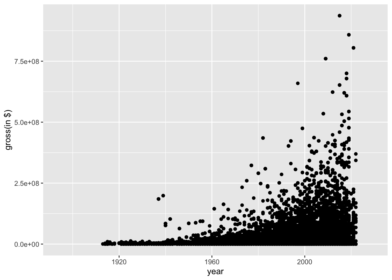
• Aplicação: Mostra a relação entre duas variáveis quantitativas.

filmes %>% # Carregar o banco
  ggplot() + ## Chamar o ggplot
  aes( x = year, y = `gross(in $)`) + ## aplicar a estética, isto é, quais são as variáveis e o que elas significam, x e y, neste caso
  geom_point() # Fazer o scatterplot

Warning: Removed 343261 rows containing missing values or values outside the scale range
(`geom_point()`).

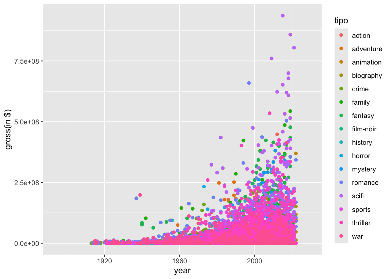
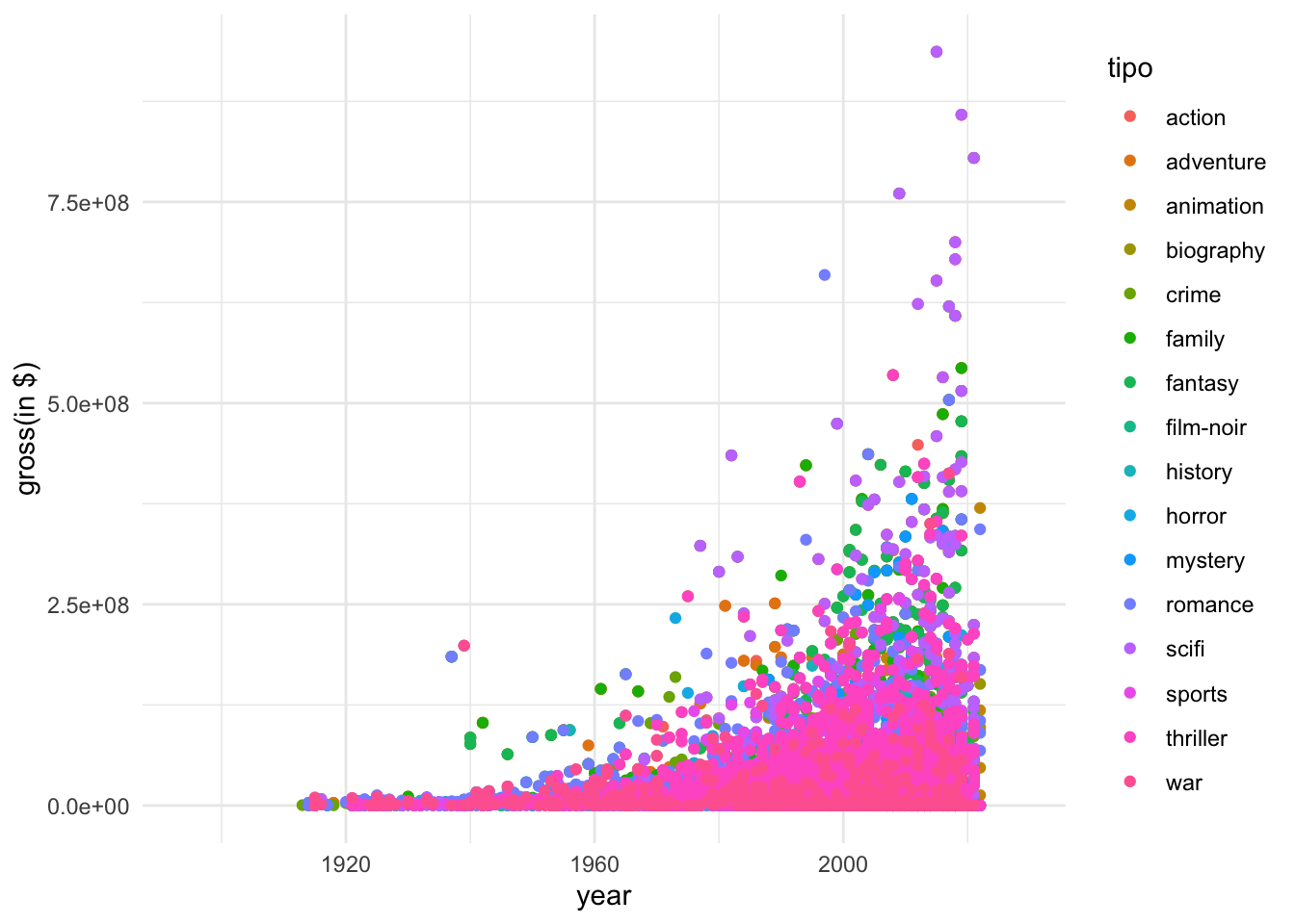
Podemos incluir a cor dos pontos, mudando a estética do gráfico.

filmes %>% 
  ggplot() +
  aes( x = year, 
       y = `gross(in $)`, 
       color = tipo) + ## Adicionamos cor
  geom_point()

Warning: Removed 343261 rows containing missing values or values outside the scale range
(`geom_point()`).

filmes %>% 
  ggplot() +
  aes( x = year, 
       y = `gross(in $)`, 
       color = tipo) + 
  geom_point() + 
  theme_minimal() ## Incluímos tema

Warning: Removed 343261 rows containing missing values or values outside the scale range
(`geom_point()`).

filmes %>% 
  ggplot() +
  aes( x = year, 
       y = `gross(in $)`, 
       color = tipo) + 
  geom_point() + 
  facet_wrap(vars(tipo)) + ## Fazemos o gráfico separado por tipo
  theme_minimal()

Warning: Removed 343261 rows containing missing values or values outside the scale range
(`geom_point()`).

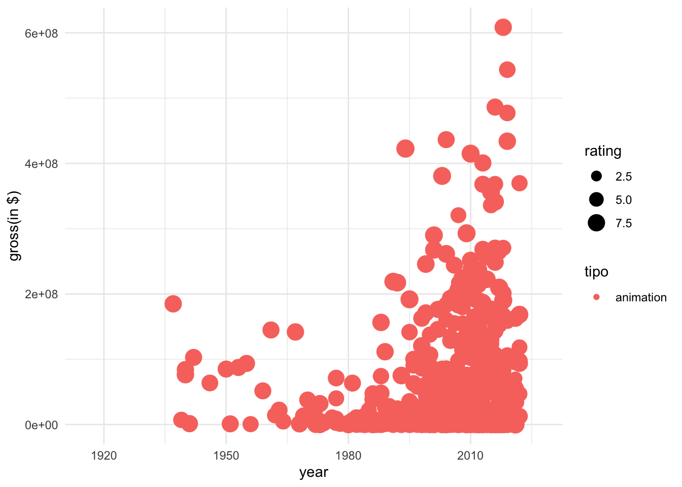
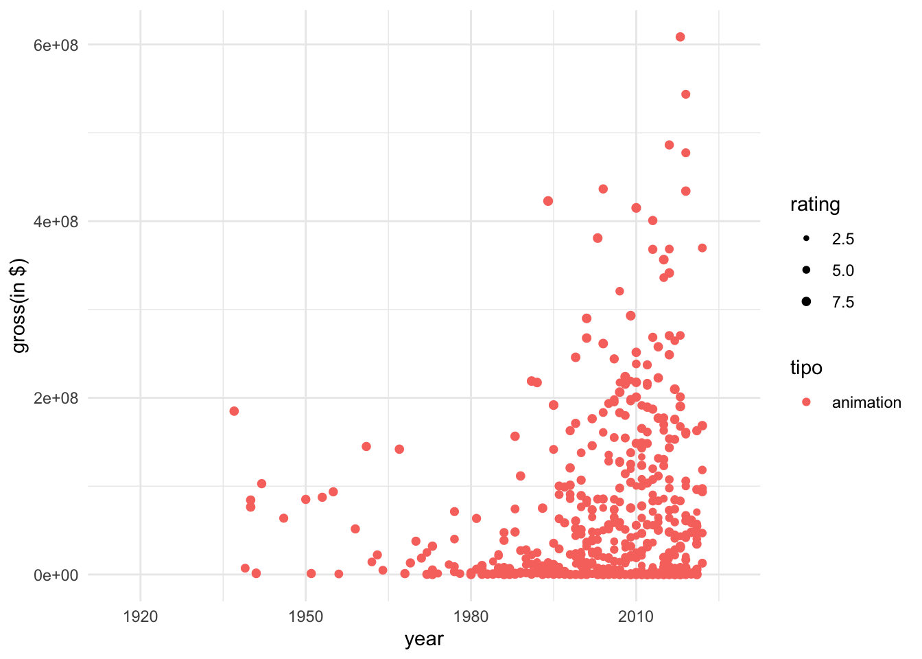
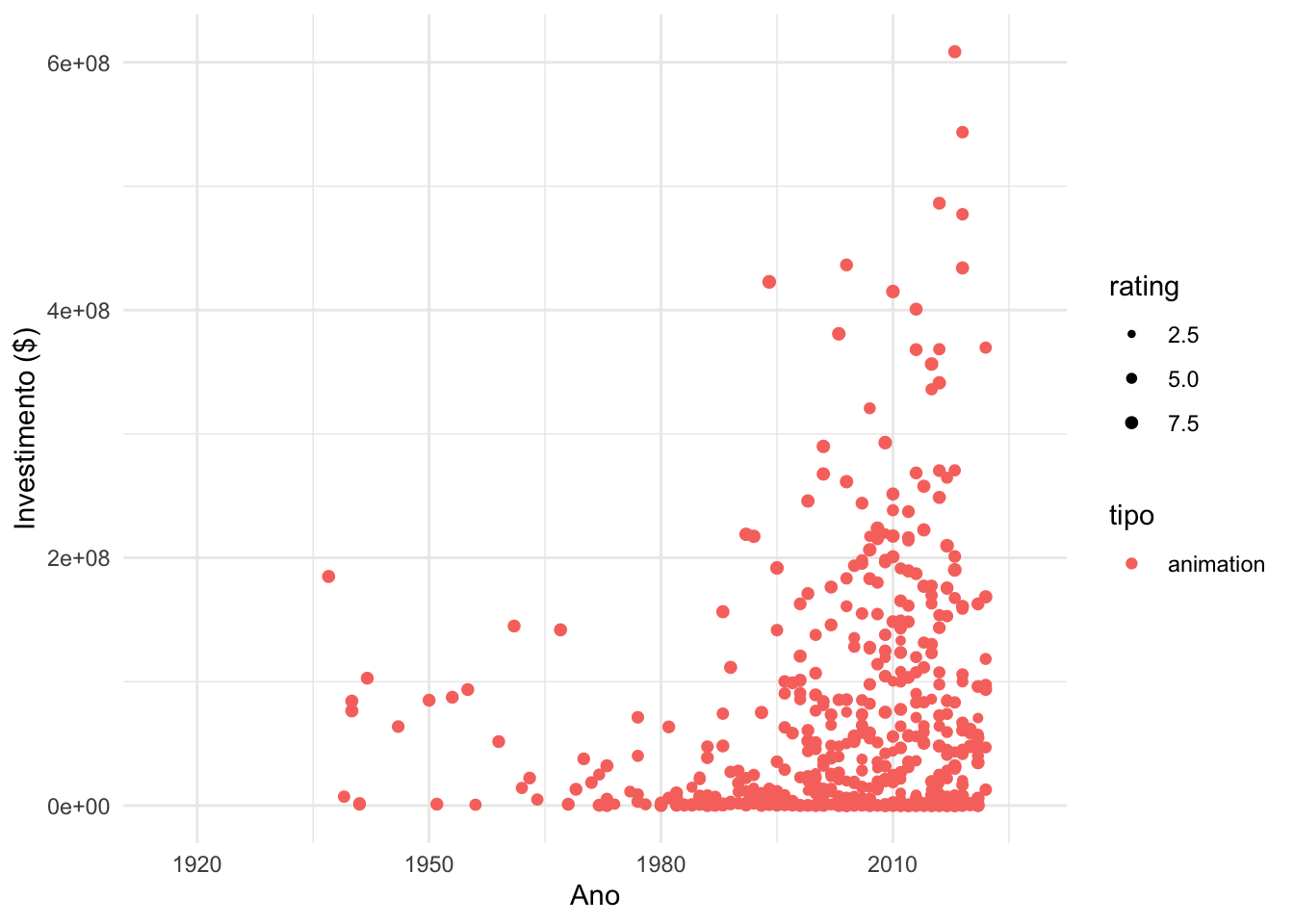
Suponha que tenhamos interesse em que o tamanho dos pontos estejam relacionados com o rating do filme. Vamos fazer isso, agora, apenas para os filmes de animação.

filmes %>% 
  filter(tipo %in% "animation") %>% 
  ggplot() +
  aes( x = year, 
       y = `gross(in $)`, 
       color = tipo, 
       size = rating) + 
  geom_point() + 
  theme_minimal()

Warning: Removed 7845 rows containing missing values or values outside the scale range
(`geom_point()`).

Para ajustarmos a escala dos pontos, basta adcionarmos uma camada de scale_size.

filmes %>% 
  filter(tipo %in% "animation") %>% 
  ggplot() +
  aes( x = year, 
       y = `gross(in $)`, 
       color = tipo, 
       size = rating) + 
  geom_point() + 
  scale_size_continuous(range=c(0.01, 2)) + 
  theme_minimal()

Warning: Removed 7845 rows containing missing values or values outside the scale range
(`geom_point()`).

Podemos alterar os nomes nos eixos utilizando a função labs.

filmes %>% 
  filter(tipo %in% "animation") %>% 
  ggplot() +
  aes( x = year, 
       y = `gross(in $)`, 
       color = tipo, 
       size = rating) + 
  geom_point() + 
  scale_size_continuous(range=c(0.01, 2)) + 
  labs(x = "Ano", 
       y = "Investimento ($)") + 
  theme_minimal()

Warning: Removed 7845 rows containing missing values or values outside the scale range
(`geom_point()`).

Para incluírmos uma linha de tendência no gráfico podemos utilizar a função geom_smooth.

filmes %>% 
  filter(tipo %in% "animation") %>% 
  ggplot() +
  aes( x = year, 
       y = `gross(in $)`, 
       color = tipo, 
       fill = tipo) + 
  geom_point() + 
  geom_smooth(method = "loess") + # O método aqui se refere ao método utilizado para estimação da curva
  scale_size_continuous(range=c(0.01, 2)) + 
  labs(x = "Ano", 
       y = "Investimento ($)") + 
  theme_minimal()

`geom_smooth()` using formula = 'y ~ x'

Warning: Removed 7845 rows containing non-finite outside the scale range
(`stat_smooth()`).

Warning: Removed 7845 rows containing missing values or values outside the scale range
(`geom_point()`).

7.1.2 Gráfico de Linhas

• Aplicação: Mostra a relação entre duas variáveis quantitativas.

filmes %>% 
  group_by(year, tipo) %>% 
  summarise(Valor_Gasto_Medio = mean(`gross(in $)`, na.rm = TRUE)) %>%
  ggplot() +
  aes( x = year, 
       y = Valor_Gasto_Medio, 
       color = tipo) + 
  geom_line() + 
  facet_wrap(vars(tipo)) + 
  theme_minimal()

`summarise()` has grouped output by 'year'. You can override using the
`.groups` argument.

Warning: Removed 222 rows containing missing values or values outside the scale range
(`geom_line()`).

filmes %>% 
  group_by(year) %>% 
  summarise(Valor_Gasto_Medio = mean(`gross(in $)`, na.rm = TRUE)) %>%
  ggplot() +
  aes( x = year, 
       y = Valor_Gasto_Medio) + 
  geom_line(alpha = 0.2) + ## Alteramos a transparencia da linha
  geom_point() + ## Colocamos Pontos
  theme_minimal()

Warning: Removed 18 rows containing missing values or values outside the scale range
(`geom_line()`).

Warning: Removed 19 rows containing missing values or values outside the scale range
(`geom_point()`).

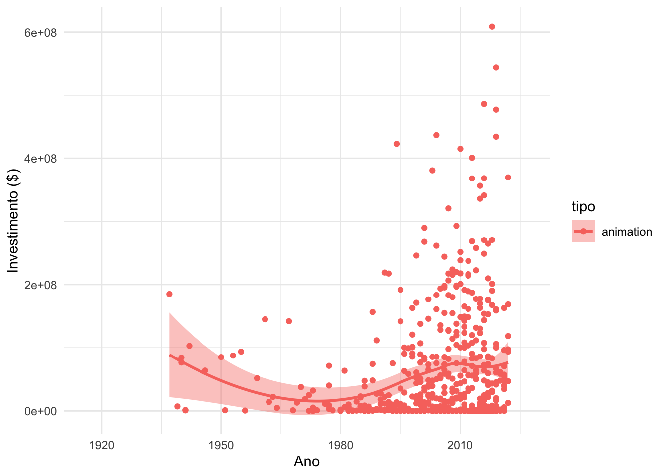
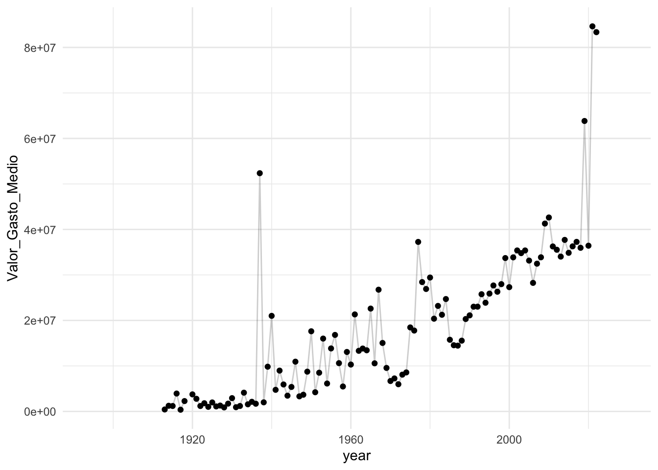
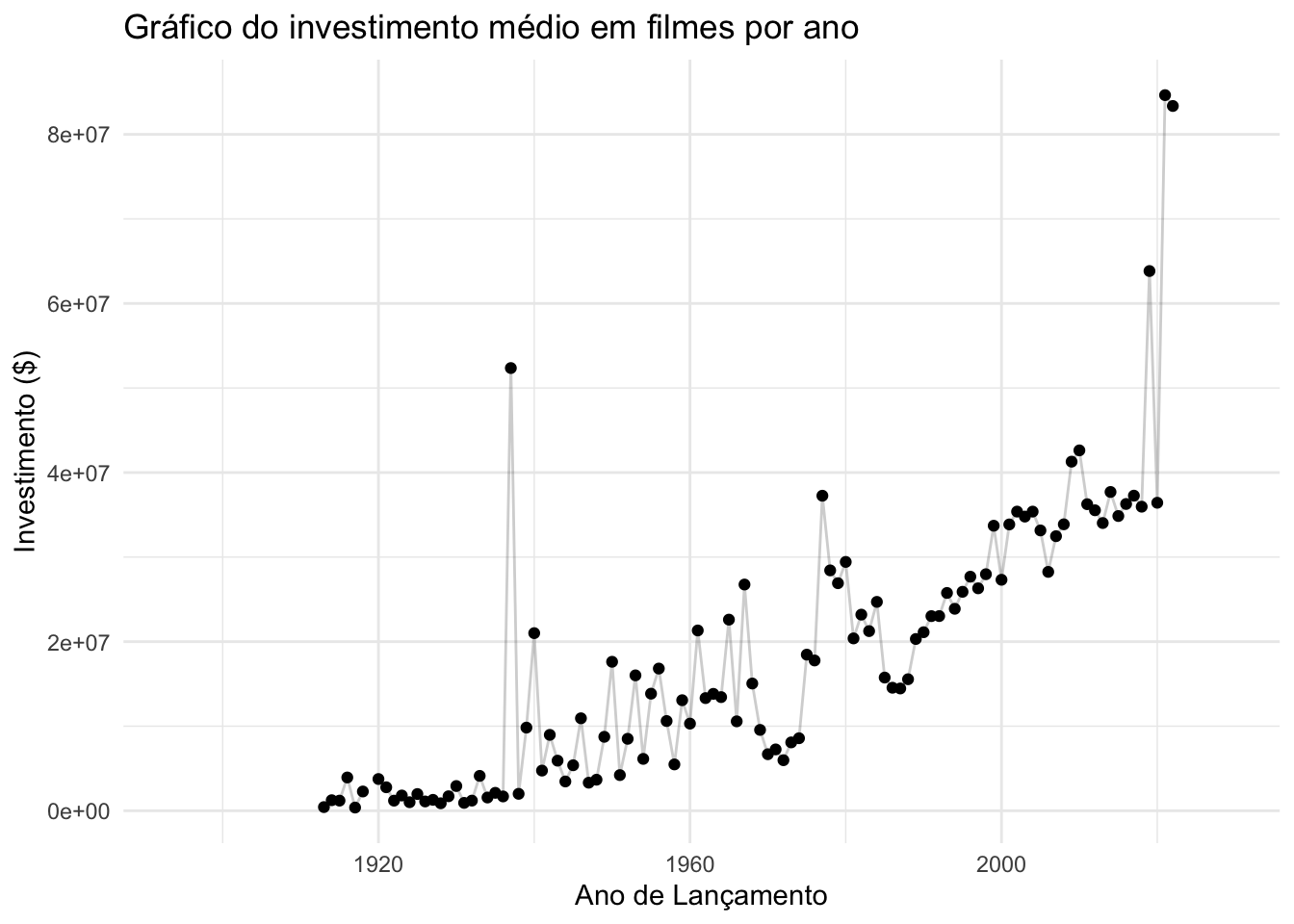
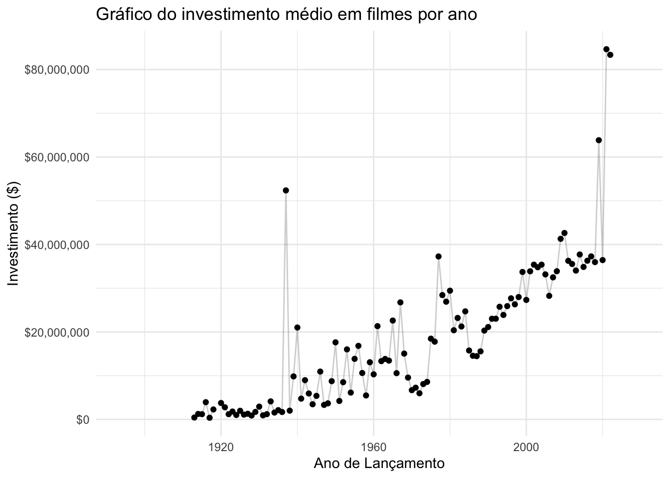
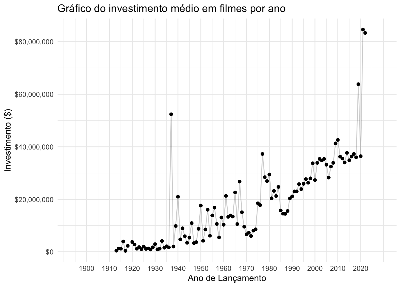
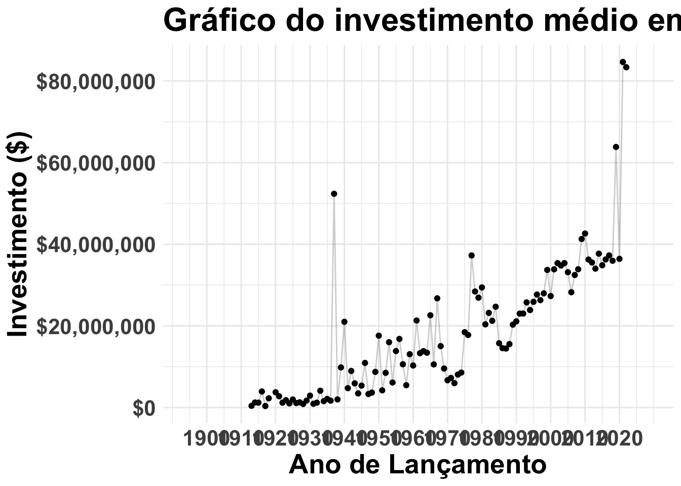
filmes %>% 
  group_by(year) %>% 
  summarise(Valor_Gasto_Medio = mean(`gross(in $)`, na.rm = TRUE)) %>%
  ggplot() +
  aes( x = year, 
       y = Valor_Gasto_Medio) + 
  geom_line(alpha = 0.2) + ## Alteramos a transparencia da linha
  geom_point() + ## Colocamos Pontos
  labs(x = "Ano de Lançamento", 
       y = "Investimento ($)", 
       title = "Gráfico do investimento médio em filmes por ano") + 
  theme_minimal()

Warning: Removed 18 rows containing missing values or values outside the scale range
(`geom_line()`).

Warning: Removed 19 rows containing missing values or values outside the scale range
(`geom_point()`).

filmes %>% 
  group_by(year) %>% 
  summarise(Valor_Gasto_Medio = mean(`gross(in $)`, na.rm = TRUE)) %>%
  ggplot() +
  aes( x = year, 
       y = Valor_Gasto_Medio) + 
  geom_line(alpha = 0.2) + 
  geom_point() + 
  labs(x = "Ano de Lançamento", 
       y = "Investimento ($)", 
       title = "Gráfico do investimento médio em filmes por ano") + 
  scale_y_continuous(labels = scales::label_dollar()) + 
  theme_minimal()

Warning: Removed 18 rows containing missing values or values outside the scale range
(`geom_line()`).

Warning: Removed 19 rows containing missing values or values outside the scale range
(`geom_point()`).

filmes %>% 
  group_by(year) %>% 
  summarise(Valor_Gasto_Medio = mean(`gross(in $)`, na.rm = TRUE)) %>%
  ggplot() +
  aes( x = year, 
       y = Valor_Gasto_Medio) + 
  geom_line(alpha = 0.2) + 
  geom_point() + 
  labs(x = "Ano de Lançamento", 
       y = "Investimento ($)", 
       title = "Gráfico do investimento médio em filmes por ano") + 
  scale_y_continuous(labels = scales::label_dollar()) + ## Alterando o label dos eixos y e x
  scale_x_continuous(breaks = seq(from = 1900, to = 2020, by = 10)) + 
  theme_minimal()

Warning: Removed 18 rows containing missing values or values outside the scale range
(`geom_line()`).

Warning: Removed 19 rows containing missing values or values outside the scale range
(`geom_point()`).

filmes %>% 
  group_by(year) %>% 
  summarise(Valor_Gasto_Medio = mean(`gross(in $)`, na.rm = TRUE)) %>%
  ggplot() +
  aes( x = year, 
       y = Valor_Gasto_Medio) + 
  geom_line(alpha = 0.2) + 
  geom_point() + 
  labs(x = "Ano de Lançamento", 
       y = "Investimento ($)", 
       title = "Gráfico do investimento médio em filmes por ano") + 
  scale_y_continuous(labels = scales::label_dollar()) +
  scale_x_continuous(breaks = seq(from = 1900, to = 2020, by = 10)) + 
  theme_minimal() +
  theme(text = element_text(size = 20, 
                            hjust = 0.5, 
                            face = "bold")) # tamanho da fonte

Warning: Removed 18 rows containing missing values or values outside the scale range
(`geom_line()`).

Warning: Removed 19 rows containing missing values or values outside the scale range
(`geom_point()`).

filmes %>% 
  group_by(year) %>% 
  summarise(Valor_Gasto_Medio = mean(`gross(in $)`, na.rm = TRUE), 
            n_filmes = n()) %>%
  ggplot() +
  aes( x = year, 
       y = Valor_Gasto_Medio) + 
  geom_line(alpha = 0.2) + 
  geom_point(aes(size = n_filmes)) + 
  labs(x = "Ano de Lançamento", 
       y = "Investimento ($)", 
       title = "Gráfico do investimento médio em filmes por ano") + 
  scale_y_continuous(labels = scales::label_dollar()) +
  scale_x_continuous(breaks = seq(from = 1900, to = 2020, by = 10)) + 
  theme_minimal() +
  theme(text = element_text(size = 20, 
                            hjust = 0.5, 
                            face = "bold")) # tamanho da fonte

Warning: Removed 18 rows containing missing values or values outside the scale range
(`geom_line()`).

Warning: Removed 19 rows containing missing values or values outside the scale range
(`geom_point()`).

filmes %>% 
  group_by(year) %>% 
  summarise(Valor_Gasto_Medio = mean(`gross(in $)`, na.rm = TRUE), 
            n_filmes = n()) %>%
  ggplot() +
  aes( x = year, 
       y = Valor_Gasto_Medio) + 
  geom_line(alpha = 0.2) + 
  geom_point(aes(size = n_filmes)) + 
  labs(x = "Ano de Lançamento", 
       y = "Investimento ($)", 
       title = "Gráfico do investimento médio em filmes por ano") + 
  scale_y_continuous(labels = scales::label_dollar()) +
  scale_x_continuous(breaks = seq(from = 1900, to = 2020, by = 10)) + 
  scale_size_continuous(range = c(0.1, 10)) + 
  theme_minimal() +
  theme(text = element_text(size = 20, 
                            hjust = 0.5, 
                            face = "bold")) # tamanho da fonte

Warning: Removed 18 rows containing missing values or values outside the scale range
(`geom_line()`).

Warning: Removed 19 rows containing missing values or values outside the scale range
(`geom_point()`).

filmes %>% 
  group_by(year) %>% 
  summarise(Valor_Gasto_Medio = mean(`gross(in $)`, na.rm = TRUE), 
            n_filmes = n()) %>%
  ggplot() +
  aes( x = year, 
       y = Valor_Gasto_Medio) + 
  geom_line(alpha = 0.2) + 
  geom_point(aes(size = n_filmes)) + 
  labs(x = "Ano de Lançamento", 
       y = "Investimento ($)", 
       title = "Gráfico do investimento médio em filmes por ano") + 
  scale_y_continuous(labels = scales::label_dollar(),
                     trans = "log10") +
  scale_x_continuous(breaks = seq(from = 1900, to = 2020, by = 10)) + 
  scale_size_continuous(range = c(0.1, 10)) + 
  theme_minimal() +
  theme(text = element_text(size = 20, 
                            hjust = 0.5, 
                            face = "bold")) # tamanho da fonte

Warning: Removed 18 rows containing missing values or values outside the scale range
(`geom_line()`).

Warning: Removed 19 rows containing missing values or values outside the scale range
(`geom_point()`).

7.1.3 Gráfico de barras

Aplicação: Comparação de categorias em um eixo categórico.

filmes %>% 
  group_by(tipo) %>% 
  summarise(Total_Investido = sum(`gross(in $)`, na.rm = TRUE)) %>%
  mutate(tipo = reorder(tipo, Total_Investido)) %>% 
  ggplot() +
  aes( x = tipo, 
       y = Total_Investido, 
       color = tipo, 
       fill = tipo) +
  geom_col() + 
  scale_y_continuous(labels = scales::label_dollar()) +
  coord_flip() +
  labs(x = "Tipo de Filme", 
       y = "Total Investido ($)") + 
  theme_minimal()

filmes %>% 
  group_by(tipo) %>% 
  summarise(Total_Investido = sum(`gross(in $)`, na.rm = TRUE)) %>%
  mutate(tipo = reorder(tipo, Total_Investido)) %>% 
  ggplot() +
  aes( x = tipo, 
       y = Total_Investido, 
       color = tipo, 
       fill = tipo) +
  geom_col(alpha = 0.2, 
           ltw = 2) + 
  scale_y_continuous(labels = scales::label_dollar()) +
  coord_flip() +
  labs(x = "Tipo de Filme", 
       y = "Total Investido ($)") + 
  theme_minimal() +
  theme(legend.position = "none")

Warning in geom_col(alpha = 0.2, ltw = 2): Ignoring unknown parameters: `ltw`

filmes %>% 
  mutate(tipo = stringr::str_to_title(tipo)) %>% 
  mutate(ano_categorico = case_when(year < 1900 ~ "< 1900", 
                                    year < 1925 ~ "< 1925", 
                                    year < 1950 ~ "< 1950", 
                                    year < 1975 ~ "< 1975", 
                                    year < 2000 ~ "< 2000", 
                                    year < 2025 ~ "< 2025")) %>%
  group_by(tipo, ano_categorico) %>% 
  summarise(Total_Investido = sum(`gross(in $)`, na.rm = TRUE)) %>%
  ungroup() %>% 
  group_by(tipo) %>% 
  mutate(total = sum(Total_Investido, na.rm = TRUE)) %>%
  ggplot() +
  aes( x = reorder(tipo, total), 
       y = Total_Investido, 
       color = ano_categorico, 
       fill = ano_categorico) +
  geom_col() + 
  scale_y_continuous(labels = scales::label_dollar()) +
  scale_color_manual(values = colorRampPalette(c("Blue", "Pink"))(7)) + 
  scale_fill_manual(values = colorRampPalette(c("Blue", "Pink"))(7)) + 
  
  coord_flip() +
  labs(x = "Tipo de Filme", 
       y = "Total Investido ($)",
       color = "Ano", 
       fill = "Ano") + 
  theme_minimal() +
  theme(legend.position = "bottom", 
        text = element_text(size = 18))

`summarise()` has grouped output by 'tipo'. You can override using the
`.groups` argument.

7.1.4 Histograma

• Aplicação: Visualização da distribuição de uma variável numérica.

ggplot(filmes) +
  aes(x = rating) +
  geom_histogram(bins = 100, fill = "#555555") +
  theme_minimal()

Warning: Removed 137362 rows containing non-finite outside the scale range
(`stat_bin()`).

ggplot(filmes) +
  aes(x = rating, fill = tipo) +
  geom_histogram(bins = 100, na.rm = TRUE) +
  theme_minimal() +
  theme(legend.position = "bottom")

7.1.5 Densidade

ggplot(filmes) +
  aes(x = rating) +
  geom_density() +
  theme_minimal() +
  theme(legend.position = "bottom")

Warning: Removed 137362 rows containing non-finite outside the scale range
(`stat_density()`).

ggplot(filmes) +
  aes(x = rating, fill = tipo, color = tipo) +
  geom_density(alpha = 0.1) +
  theme_minimal() +
  theme(legend.position = "bottom")

Warning: Removed 137362 rows containing non-finite outside the scale range
(`stat_density()`).

ggplot(filmes) +
  aes(x = rating, fill = tipo, color = tipo) +
  geom_density(alpha = 0.1) +
  facet_wrap(vars(tipo)) + 
  theme_minimal() +
  theme(legend.position = "none")

Warning: Removed 137362 rows containing non-finite outside the scale range
(`stat_density()`).

7.1.6 Boxplot

• Aplicação: Visualização da distribuição de uma variável numérica.

ggplot(filmes) +
  aes(x = rating, fill = tipo, color = tipo) +
  geom_boxplot(alpha = 0.1) +
  theme_minimal() +
  theme(legend.position = "none")

Warning: Removed 137362 rows containing non-finite outside the scale range
(`stat_boxplot()`).

ggplot(filmes) +
  aes(x = rating, 
      y = tipo, 
      fill = tipo, 
      color = tipo) +
  geom_boxplot(alpha = 0.1, 
               outlier.shape = NA) +
  geom_jitter(size = 0.1, 
              alpha = 0.1, 
              pch = 20) + 
  theme_minimal() +
  theme(legend.position = "none")

Warning: Removed 137362 rows containing non-finite outside the scale range
(`stat_boxplot()`).

Warning: Removed 137362 rows containing missing values or values outside the scale range
(`geom_point()`).

7.1.7 Gráfico de Violino

• Aplicação: Visualização da distribuição de uma variável numérica.

ggplot(filmes) +
  aes(x = rating, y = tipo, color = tipo) +
  geom_violin(alpha = 0.1) +
  theme_minimal() +
  theme(legend.position = "none")

Warning: Removed 137362 rows containing non-finite outside the scale range
(`stat_ydensity()`).

ggplot(filmes) +
  aes(x = rating, y = 1) +
  geom_violin(alpha = 0.1) +
  geom_boxplot() + 
  theme_minimal() +
  theme(legend.position = "none")

Warning: Removed 137362 rows containing non-finite outside the scale range
(`stat_ydensity()`).

Warning: Removed 137362 rows containing non-finite outside the scale range
(`stat_boxplot()`).

ggplot(filmes) +
  aes(x = rating, y = 1) +
  geom_violin(alpha = 0.1) +
  geom_boxplot(width = 0.4) + 
  theme_minimal() +
  theme(legend.position = "none")

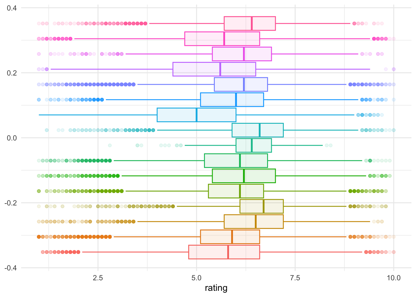
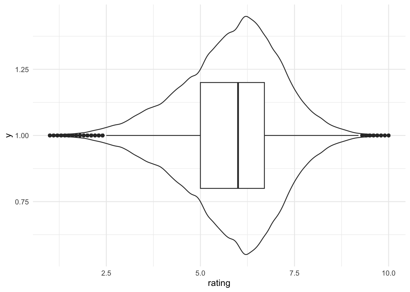
Warning: Removed 137362 rows containing non-finite outside the scale range
(`stat_ydensity()`).
Removed 137362 rows containing non-finite outside the scale range
(`stat_boxplot()`).

7.2 Adições ao ggplot2 & outros procedimentos gráficos

7.2.1 Gráficos de Dispersão Hexagonais

O geom_hex é útil para criar gráficos de dispersão hexagonais. Esses gráficos são úteis quando você deseja representar dados de alta densidade em um gráfico de dispersão, especialmente quando há muitos pontos que se sobrepõem.

filmes %>%
  filter(tipo %in% "animation") %>% 
  ggplot() + 
  aes(x = rating, y = year) + 
  geom_hex(bins = 20, 
           color = "white", 
           size = 2) +
  scale_fill_gradient(low = "#FED0BB",
                      high = "#461220", 
                      guide = FALSE) + 
  coord_flip() + 
  theme_minimal()

Warning: Using `size` aesthetic for lines was deprecated in ggplot2 3.4.0.
ℹ Please use `linewidth` instead.

Warning: Removed 3658 rows containing non-finite outside the scale range
(`stat_binhex()`).

Warning: Computation failed in `stat_binhex()`.
Caused by error in `compute_group()`:
! The package "hexbin" is required for `stat_bin_hex()`.

Warning: The `guide` argument in `scale_*()` cannot be `FALSE`. This was deprecated in
ggplot2 3.3.4.
ℹ Please use "none" instead.

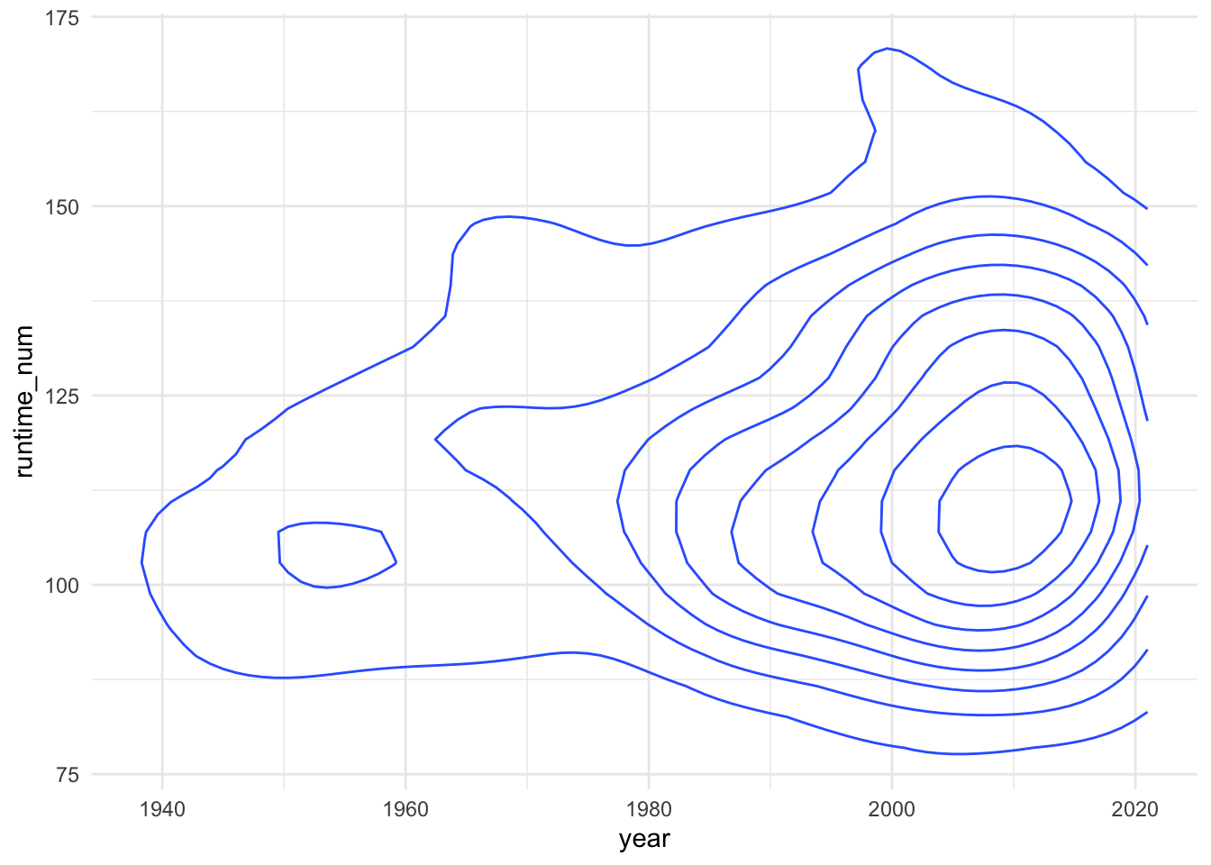
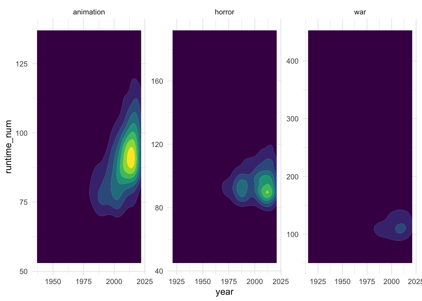
7.2.2 Gráfico de Contorno

O geom_contour é uma camada geométrica do pacote ggplot2 em R que é usada para criar gráficos de contorno. Os gráficos de contorno são usados para visualizar a densidade de pontos em um espaço bidimensional, onde as linhas de contorno representam regiões de densidade semelhante. Isso é útil quando você deseja identificar padrões de densidade em um gráfico de dispersão ou mapa.

filmes %>%
  filter(tipo %in% "war") %>% 
  mutate(runtime_num = stringr::str_remove(runtime, "min") %>% 
           str_squish() %>% 
           as.numeric()) %>% 
  filter(!is.na(runtime_num)) %>% 
  filter(`gross(in $)` > 0 | !is.na(`gross(in $)`)) %>% 
  ggplot() + 
  aes(x = year, 
      y = runtime_num) + 
  geom_density_2d() +
  theme_minimal() + 
  theme(legend.position = "none")

filmes %>%
  filter(tipo %in% c("war", "animation", "horror")) %>%
  mutate(runtime_num = stringr::str_remove(runtime, "min") %>% 
           str_squish() %>% 
           as.numeric()) %>% 
  filter(!is.na(runtime_num)) %>% 
  filter(`gross(in $)` > 0 | !is.na(`gross(in $)`)) %>% 
  ggplot() + 
  aes(x = year, 
      y = runtime_num) + 
  geom_density_2d_filled(contour_var = "density") +
  theme_minimal() + 
  theme(legend.position = "none") +
  facet_wrap(vars(tipo), scales = "free")

Warning: There was 1 warning in `mutate()`.
ℹ In argument: `runtime_num = stringr::str_remove(runtime, "min") %>%
  str_squish() %>% as.numeric()`.
Caused by warning in `stringr::str_remove(runtime, "min") %>% str_squish() %>% as.numeric()`:
! NAs introduced by coercion

7.3 Utilizando o pacote esquisse

Uma opção para facilitar a utilização do pacote ggplot2 é utilizarmos o addin esquisse. A utilização do pacote permite a criação de um gráfico base que podemos personalizar em seguir.

7.3.1 Adcionando labels nos gráficos

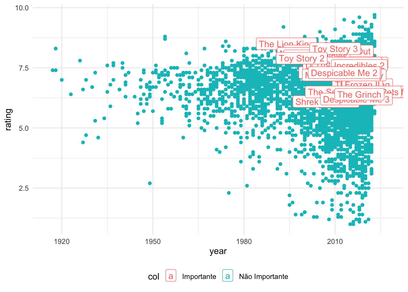
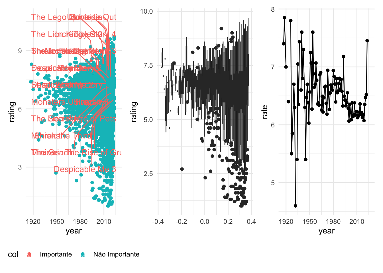
Muitas vezes temos interesse em incluir alguma informação no nosso gráfico, seja ela por meio de um texto ou anotação. Uma maneira simples e rápida para fazermos isso é pelo uso da estética label e o geom_text.

filmes %>% 
  filter(tipo %in% c("animation")) %>% 
  mutate(nome = ifelse(`gross(in $)` > quantile(`gross(in $)`, 0.95, na.rm = T), movie_name, NA)) %>% 
  mutate(col = ifelse(!is.na(nome), "Importante", "Não Importante")) %>%
  ggplot() +
  aes(x = year, 
      y = rating, 
      label = nome, 
      color = col)+
  geom_point() +
  geom_label() +
  theme_minimal() +
  theme(legend.position = "bottom")

Warning: Removed 3658 rows containing missing values or values outside the scale range
(`geom_point()`).

Warning: Removed 8390 rows containing missing values or values outside the scale range
(`geom_label()`).

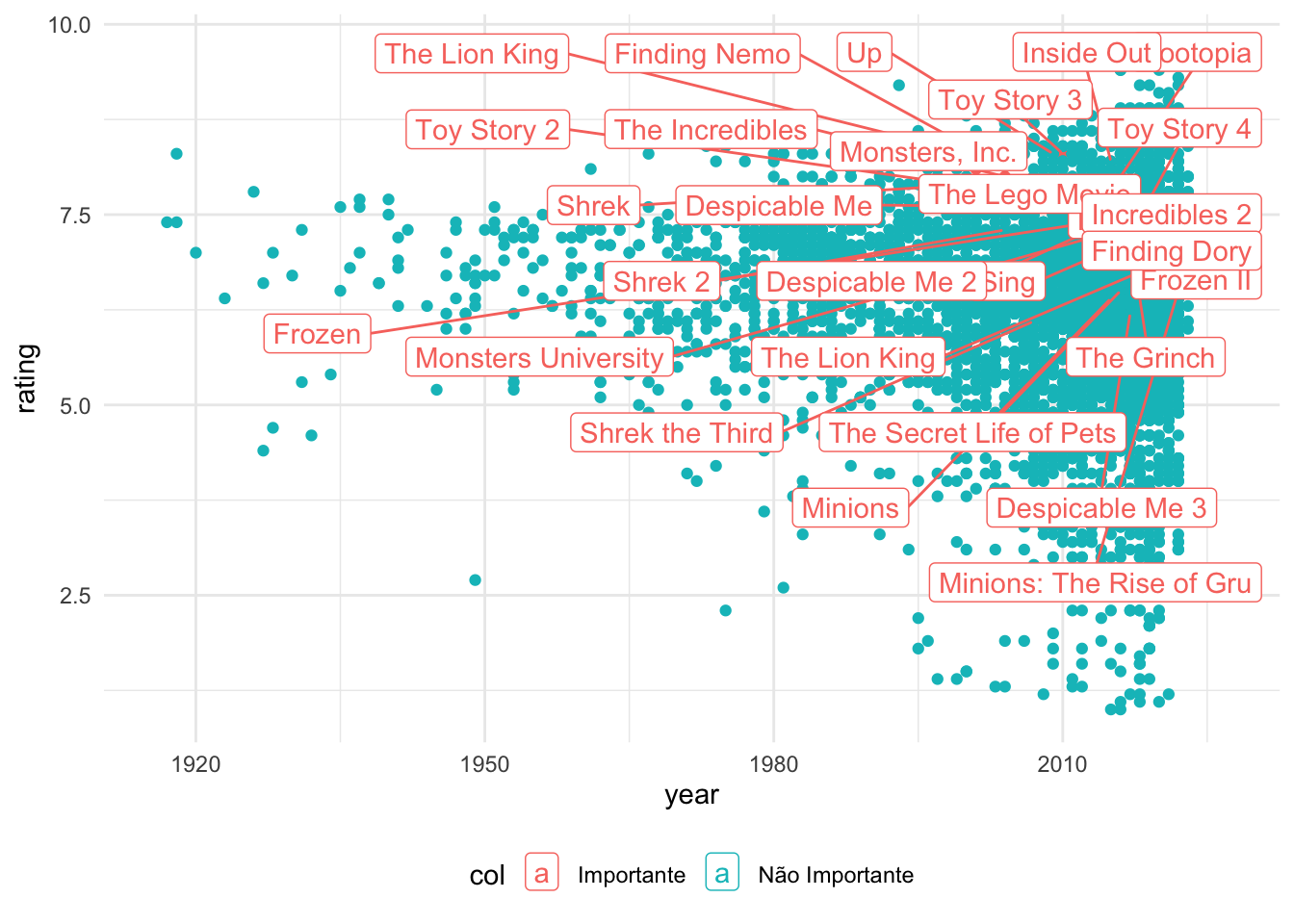
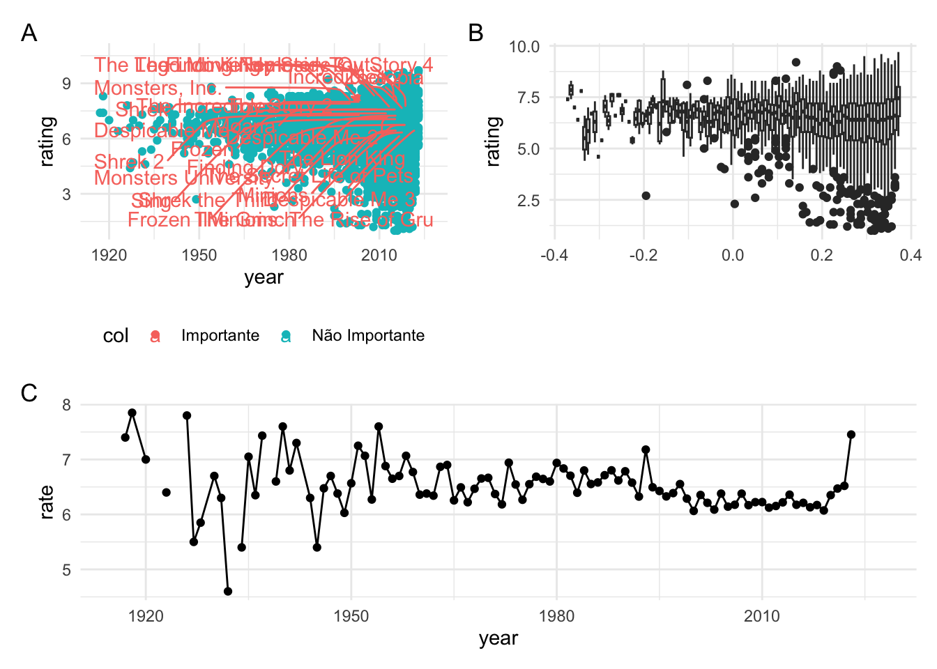
Contudo, nem sempre é possível incluirmos os labels dessa maneira. A extensão ggrepel é uma alternativa, permitindo que vários labels seja adcionados sem sobreposição.

require(ggrepel)

Loading required package: ggrepel

filmes %>% 
  filter(tipo %in% c("animation")) %>% 
  mutate(nome = ifelse(`gross(in $)` > quantile(`gross(in $)`, 0.95, na.rm = T), movie_name, NA)) %>% 
  mutate(col = ifelse(!is.na(nome), "Importante", "Não Importante")) %>%
  ggplot() +
  aes(x = year, 
      y = rating, 
      label = nome, 
      color = col)+
  geom_point() +
  geom_label_repel(box.padding = 0.5, 
                   max.overlaps = 1000) +
  theme_minimal() +
  theme(legend.position = "bottom")

Warning: Removed 3658 rows containing missing values or values outside the scale range
(`geom_point()`).

Warning: Removed 8390 rows containing missing values or values outside the scale range
(`geom_label_repel()`).

filmes %>% 
  filter(tipo %in% c("animation")) %>% 
  mutate(nome = ifelse(`gross(in $)` > quantile(`gross(in $)`, 0.95, na.rm = T), movie_name, NA)) %>% 
  mutate(col = ifelse(!is.na(nome), "Importante", "Não Importante")) %>%
  ggplot() +
  aes(x = year, 
      y = rating, 
      label = nome, 
      color = col)+
  geom_point() +
  geom_text_repel(box.padding = 0.5, 
                  max.overlaps = 1000, 
                  nudge_x = .15,
                  nudge_y = 1,
                  segment.curvature = -0.1,
                  segment.ncp = 3,
                  segment.angle = 20
  ) +
  theme_minimal() +
  theme(legend.position = "bottom")

Warning: Removed 3658 rows containing missing values or values outside the scale range
(`geom_point()`).

Warning: Removed 8390 rows containing missing values or values outside the scale range
(`geom_text_repel()`).

7.4 Layouts

Muitas vezes precisamos colocar diversos gráficos em uma mesma página. Para isso, podemos utilizar diversos pacotes como o cowplot e o patchwork.

require(patchwork)

Loading required package: patchwork

p1 = 
  filmes %>% 
  filter(tipo %in% c("animation")) %>% 
  mutate(nome = ifelse(`gross(in $)` > quantile(`gross(in $)`, 0.95, na.rm = T), movie_name, NA)) %>% 
  mutate(col = ifelse(!is.na(nome), "Importante", "Não Importante")) %>%
  ggplot() +
  aes(x = year, 
      y = rating, 
      label = nome, 
      color = col)+
  geom_point() +
  geom_text_repel(box.padding = 0.5, 
                  max.overlaps = 1000, 
                  nudge_x = .15,
                  nudge_y = 1,
                  segment.curvature = -0.1,
                  segment.ncp = 3,
                  segment.angle = 20
  ) +
  theme_minimal() +
  theme(legend.position = "bottom")

p2 = filmes %>% 
  filter(tipo %in% c("animation")) %>% 
  ggplot() +
  aes(group = year, 
      y = rating, 
  )+
  geom_boxplot() +
  theme_minimal() +
  theme(legend.position = "bottom")

p3 = filmes %>% 
  filter(tipo %in% c("animation")) %>% 
  group_by(year) %>% 
  summarise(rate = mean(rating, na.rm = TRUE)) %>% 
  ggplot()+
  aes(x = year, 
      y = rate) + 
  geom_line() +
  geom_point() +
  theme_minimal()

p1 / p2

Warning: Removed 3658 rows containing missing values or values outside the scale range
(`geom_point()`).

Warning: Removed 8390 rows containing missing values or values outside the scale range
(`geom_text_repel()`).

Warning: Removed 3658 rows containing non-finite outside the scale range
(`stat_boxplot()`).

p1 + p2 + p3

Warning: Removed 3658 rows containing missing values or values outside the scale range
(`geom_point()`).

Warning: Removed 8390 rows containing missing values or values outside the scale range
(`geom_text_repel()`).

Warning: Removed 3658 rows containing non-finite outside the scale range
(`stat_boxplot()`).

Warning: Removed 5 rows containing missing values or values outside the scale range
(`geom_line()`).

Warning: Removed 10 rows containing missing values or values outside the scale range
(`geom_point()`).

(p1 + p2 )/(p3) + plot_annotation(tag_levels = "A")

Warning: Removed 3658 rows containing missing values or values outside the scale range
(`geom_point()`).

Warning: Removed 8390 rows containing missing values or values outside the scale range
(`geom_text_repel()`).

Warning: Removed 3658 rows containing non-finite outside the scale range
(`stat_boxplot()`).

Warning: Removed 5 rows containing missing values or values outside the scale range
(`geom_line()`).

Warning: Removed 10 rows containing missing values or values outside the scale range
(`geom_point()`).

7.4.1 Exportando gráfico

Para exportarmos um gráfico como PDF ou PNG podemos realizar o seguinte procedimento:

Cairo::CairoPDF("Caminho/nome_do_grafico.pdf")
p1
dev.off()

Cairo::CairoPNG("Caminho/nome_do_grafico.png")
p1
dev.off()

7.4.2 Gráficos Interativos

Podemos transformar qualquer gráfico do ggplot em interativo utilizando o pacote plotly.

require(plotly)

Loading required package: plotly

Attaching package: 'plotly'

The following object is masked from 'package:ggplot2':

    last_plot

The following object is masked from 'package:stats':

    filter

The following object is masked from 'package:graphics':

    layout

p3 %>%  ggplotly()

7.5 Gráficos Animados

Para fazer gráficos dinâmicos podemos utilizar o gganimate.

require(gganimate)

Loading required package: gganimate

filmes %>% 
    group_by(tipo, year) %>% 
    summarise(n = log10(n())) %>%
    group_by(year) %>% 
    mutate(Rank = rank(n)) %>%
    ggplot() + 
    aes(x = Rank, 
        y = n, 
        color = tipo, 
        fill = tipo, 
        label = tipo) +
    geom_col(show.legend = F, alpha = 0.5) + 
    geom_text(show.legend = F, nudge_y = 1 , size = 10) + 
    coord_flip() + 
    scale_y_continuous(limits  = c(0,8)) + 
    # Agora, incluimos as partes do gganimate
    labs(#title = 'Ano: {frame_time}', 
        x = 'Tipo de Filme', 
        y = 'Número de Filmes') +
    #transition_time(year) +
    ggtitle('{closest_state}') +
    transition_states(year,
                      transition_length = 5,
                      state_length = 1) +
    ease_aes('linear') + 
    theme_minimal() +  
    theme(text = element_text(size = 20)) + 
    exit_fade() +   
    enter_fade() 

`summarise()` has grouped output by 'tipo'. You can override using the
`.groups` argument.

Warning in lapply(row_vars$states, as.integer): NAs introduced by coercion
Warning in lapply(row_vars$states, as.integer): NAs introduced by coercion

Warning in expand_panel(..., self = self): NAs introduced by coercion
Warning in expand_panel(..., self = self): NAs introduced by coercion

7.6 Exercício

1. Faça pelo menos cinco gráficos (distintos), utilizando os diferentes dados apresentados no conjunto de dados filmes.
2. Combine os gráficos em uma página e salve em um pdf.
3. Crie um gráfico animado.